Implementing k Nearest Neighbours from scratch in Python

This post is a follow up from the previous post. I will work through an implementation from scratch in python.

The code is saved at my github.

The data

The data is a well known dataset related to features of Iris flowers, from the Iris Plants Database. It might be the best known dataset in classification literature, related to several classic papers. The data is here, and more info on the dataset is here.

The code

First, importing the dataset and having a look at the data.

# import required packages
from csv import reader
from math import sqrt

#create a simple function for loading csvs

def load_csv(filename):
    dataset = list()
    with open(filename, 'r') as file:
        csv_read = reader(file)
        for row in csv_read:
            if not row:
                continue
            dataset.append(row)
    return dataset

#identify the file name and load the data

filename = 'iris.csv'
dataset = load_csv(filename)

#view the data

#note it is all in string format and needs to be reformatted

dataset
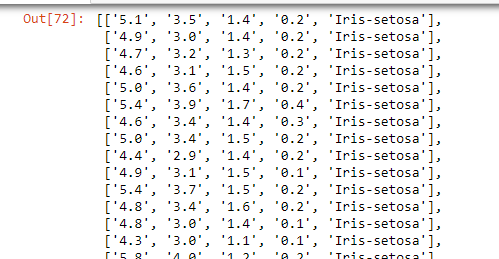
First view of the data.

Then cleaning the data, converting strings to the correct formats.

# function to convert string column to float

#strip removed trailing and leading blanks
#float function converts to float

def str_to_float(dataset, col):
    for row in dataset:
        row[col] = float(row[col].strip())

#apply the formula to all but the last column

for i in range(len(dataset[0])-1):
    str_to_float(dataset, i)

#now need to clean up the categorical variable, convert it to an integer.

def str_to_int(dataset, col):
    #identify classes
    classes = [row[col] for row in dataset]
    #get distinct classes
    distinct = set(classes)
    #initialise dictionary of class values
    lookup = dict()
    #fill dict with integer for each class value
    for i, value in enumerate(distinct):
        lookup[value] = i
        print('[%s] = %d' % (value, i))
    #lookup into the dictionary, based on the string
    for row in dataset:
        row[col] = lookup[row[col]]
    return lookup 

 #apply formula to last column
    
str_to_int(dataset, len(dataset[0])-1)
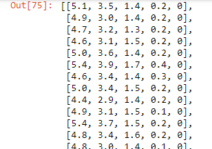
Cleaner!

The algorithm

Functions to calculate euclidean distance, identify neighbours, and apply the algorithm to new data.


# Calculate the Euclidean distance
def euclid_dist(r1, r2):
    #initialise distance
    distance = 0.0
    #loop through rows
    for i in range(len(r1)-1):
        distance += (r1[i] - r2[i])**2
    return sqrt(distance)

# Locate the most similar neighbors
def get_neighbours(train, test_row, num_neighbours):
    #train is the training dataset
    #test_row is a single observation
    #num_neighbours is the predefined k value
    
    #initialise list
    distances = list()
    #loop through train rows
    for train_row in train:
        #measure distance betweeen test row and train row
        dist = euclid_dist(test_row, train_row)
        #add train row and distance to distances dataset
        distances.append((train_row, dist))
    #sort by distance
    distances.sort(key=lambda tup: tup[1])
    neighbours = list()
    #identify top k neighbours
    for i in range(num_neighbours):
        neighbours.append(distances[i][0])
    return neighbours
 

# Make a prediction

def predict_class(train, test_row, num_neighbours):
    #identify neighbours using neighbour function
    neighbours = get_neighbours(train, test_row, num_neighbours)
    #keep the class variable
    output = [row[-1] for row in neighbours]
    #assign the most common category as the prediction
    prediction = max(set(output), key=output.count)
    return prediction
 

and then applying it to a single new input!

# define k
num_neighbours = 5
# define a new record
row = [4.3,1.1,2.2,1.1]
# predict the class
label = predict_class(dataset, row, num_neighbours)
print('Data=%s, Predicted: %s' % (row, label))

It runs!

Testing the accuracy of the algorithm

import random

random.shuffle(dataset)

train_data = dataset[:120]
test_data = dataset[120:]

num_neighbours = 5

correct = 0
for i in range(len(test_data)):
    y = predict_class(train_data, test_data[i][0:4], num_neighbours)
    if y == test_data[i][4]:
        correct += 1
    print(y, test_data[i][4])

29 out of 30 correct classifications in the test dataset. Not bad!

Algorithm Overview: k-Nearest Neighbours

k-Nearest Neighbours (k-NN) is a non-parametric classification algorithm that has been around since the 50’s. It is typically used for classification, but can also be used for evaluation. With classification, a data point is compared to the k observations closest to it, and the classes of those observations infer the class of the data point. With regression, the same approach is taken, but the mean of the regression variable is used as the inferred value for the data point. Classification is the more common use.

The measure of distance used to identify neighbours is important, as is the scales of the variables involved – if they vary significantly then standardisation can help with accuracy. Finally, weights are sometimes applied to the neighbours, with nearer data points carrying more significance.

How The Algorithm Works

The training dataset consists of multidimensional vectors, each with a class label.

The classification dataset is an unlabeled vector. With a user-defined k, the unlabeled vector is compared to its k nearest neighbours. For classification, the unlabeled vector gets the mode label from the k nearest neighbours. For regression, it gets the average of the k nearest labels.

Distance Metrics

The most commonly used distance metric for continuous variables is Euclidean Distance. In n-dimensional space the formula is:

Formula from linked Wikipedia page.

For discrete variables, including text classification, metrics like the Hamming Distance can work.

Choosing K

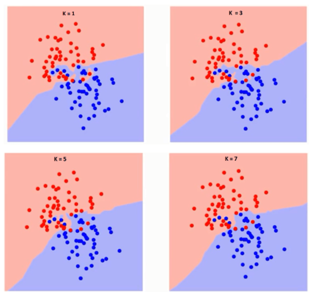
Choosing k depends on the data. Larger values of k can reduce noise, but the boundaries between classes can become complicated. Choice of features can also introduce significant noise: having irrelevant or unimportant features in the data degrades the algorithm’s performance. Feature selection and feature scaling can help with optimisation.

Running the algorithm at different values of k will allow for error rate inspection and optimal parameter choice.

Examples

Here’s a simple example that does calculations by hand.

Here’s a blog post with a from-scratch implementation in python.

Here’s a great blog post from analyticsvidhya.com with python and R implementation, and some nice graphical examples.

Graphs from analyticsvidhya’s post.

Building a Neural Network from scratch using PyTorch and FastAI

This post follows content from fastai to build a two layer Neural Network from scratch using python. The code is saved on my github.

The data, and data prep

I used a sample dataset from FastAI based on a famous computer vision dataset, MNIST. The sample dataset uses 3s and 7s only, to make the overall problem simpler.

After importing the required packages and connecting to the data, we can see some of the images in the dataset. There are over 6000 ‘3s’ in the dataset. Here are a few of them:

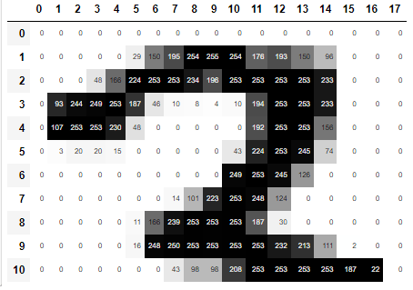
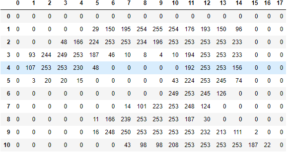
They can also be viewed as arrays, where each pixel has a value between 0 (white) and 255 (black). This is the top portion of one.

It is easier to see if the array is shaded.

Using python we can stack the images into a single tensor, and then see what the ‘average’ 3 or 7 looks like:

# creating lists of the images in the 7 and 3 folders
seven_tensors = [tensor(Image.open(o)) for o in sevens]
three_tensors = [tensor(Image.open(o)) for o in threes]
len(three_tensors),len(seven_tensors)
# using torch.stack to stack the tensors into a 3 dimensional tensor
stacked_sevens = torch.stack(seven_tensors).float()/255
stacked_threes = torch.stack(three_tensors).float()/255
stacked_threes.shape
# the average 3
mean3 = stacked_threes.mean(0)
show_image(mean3);
# the average 7
mean7 = stacked_sevens.mean(0)
show_image(mean7);
The average 3
The average 7.

Structuring the data for the Neural Net

Using PyTorch we get the data into a format and shape that works for our calculations. Our images are transformed into a tensor with 12396 rows and 784 columns. The 784 columns represent the 28 x 28 pixels, flattened. Our labels are a vector with 12396 rows and 1 column.

train_x = torch.cat([stacked_threes, stacked_sevens]).view(-1, 28*28)
train_y = tensor([1]*len(threes) + [0]*len(sevens)).unsqueeze(1)
train_x.shape,train_y.shape
The data in the correct shape and format.

The training data is put into a dataset where the x,y variables are available as a tuple. x is the 784 pixels of an image and y is the label. The same prep is applied to the validation data.

dset = list(zip(train_x,train_y))
x,y = dset[0]
x.shape,y
The prepared dataset, in tuple form.

With a set of randomly generated weights and biases, a simple linear model of the form y = ax + b is created, and when the training data is applied to it, a score for every image is output:

def linear1(xb): return xb@weights + bias
preds = linear1(train_x)
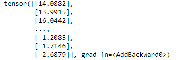
preds
The outputted scores.

Turns out this has a 57% accuracy, so not much better than guessing. This is to be expected since the weights were randomly generated.

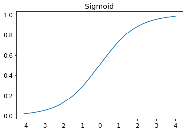
The next step should be to update the weights in a way that improves the accuracy slightly. One issue with this is that a small change in the weights might not change the accuracy at all, causing the algorithm to get stuck. Introducing the sigmoid function; It is a smooth continuous function that will always give a different output for small changes in weights. This allows us to make and measure the effect of small changes in the parameters, so that the model moves in the right direction.
Any input to the function always gives an output between 0 and 1.

Putting the model together

All in all then, we do the following:
1. Initialise a set of random weights and biases
2. Apply our training data to the model
3. Calculate the loss of the predictions compared to the correct answers
4. Calculated the gradients of the parameters and adjust the parameters
5. Go back to step 2

# This function:
#     Takes the input data
#     Makes predictions based on the model ax + b
#     Calculates the loss using the sigmoid functionality when comparing to the dependent values
#     Calculated the gradients using the .backward() method
def calc_grad(xb, yb, model):
    preds = model(xb)
    loss = mnist_loss(preds, yb)
    loss.backward()
def train_epoch(model, lr, params):
    for xb,yb in dl:
        calc_grad(xb, yb, model)
        for p in params:
            p.data -= p.grad*lr
            p.grad.zero_()
def batch_accuracy(xb, yb):
    preds = xb.sigmoid()
    correct = (preds>0.5) == yb
    return correct.float().mean()
def validate_epoch(model):
    accs = [batch_accuracy(model(xb), yb) for xb,yb in valid_dl]
    return round(torch.stack(accs).mean().item(), 4)

Running the code for 20 epochs shows increasing accuracy

for i in range(20):
    train_epoch(linear1, lr, params)
    print(validate_epoch(linear1), end=' ')
Accuracy after each epoch.

Adding Nonlinearity

Adding a nonlinear layer gives us a true neural net. Here is a tw0-layer neural net, with a RELU layer in between.

def simple_net(xb): 
    res = xb@w1 + b1
    res = res.max(tensor(0.0))
    res = res@w2 + b2
    return res

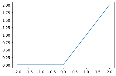
Here’s the nonlinear aspect introduced by the RELU function, visualised:

RELU

Much of this can be replaced with ready-made components from either PyTorch or fastai, making it easier to implement,

simple_net = nn.Sequential(
    nn.Linear(28*28,30),
    nn.ReLU(),
    nn.Linear(30,1)
)
learn = Learner(dls, simple_net, opt_func=SGD,
                loss_func=mnist_loss, metrics=batch_accuracy)
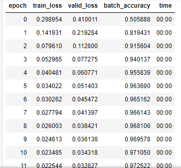
learn.fit(40, 0.1)
Output from the fastai learner.
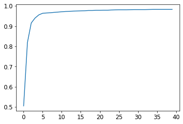
Accuracy, visualised.

The accuracy after 40 epochs is 98.2%. A quick comparison with more mature methods shows that there is still lots more to do: a single epoch of fastai’s resnet18 model gives accuracy of 99.7%!

dls = ImageDataLoaders.from_folder(path)
learn = cnn_learner(dls, resnet18, pretrained=False,
                    loss_func=F.cross_entropy, metrics=accuracy)
learn.fit_one_cycle(1, 0.1)
Output from one epoch of Resnet18

A Simple Demonstration of Gradient Descent in Python

This post looks at the concept of gradient descent, and applies it to a simple function. It is prompted by and takes some code from the fastai lesson content.
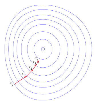
Put simply, gradient descent is used to give feedback to a deep learning model so it can adjust its parameters. The intention is to prompt the model to adjust the parameters so that the model will improve slightly, and make repeated improvements so that the model gets iteratively better.

From the wikipedia link above.

Mathematically, it is an algorithm for finding the local minimum of a differentiable function. The differentiable function in this case is the loss function of the model, and the local minimum represents the (or one of the) best set(s) of parameters for the model.

The full code for this is saved here. I’ll include highlights and graphs in this post.

First, we generate a simple dataset to train our model to.

# Define a tensor of time values
time = torch.arange(0,20).float(); time
# Define a tensor of speed values, with a quadratic element built in
speed = torch.randn(20)*2 + 0.75*(time-9.5)**2 + 1
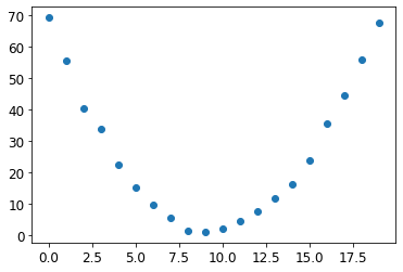
plt.scatter(time,speed);
A plot of the ‘dataset’.

Then, define a function as the basis for our model (in this case it is a quadratic function), and a loss function (mean square error).

# We base our model on a quadratic function, based on the shape of the plot
# Need to solve for a, b and c

def f(t, params):
    a,b,c = params
    return a*(t**2) + (b*t) + c

# Also define a function to measure loss. The mean squared error works.

def mse(preds, targets): return ((preds-targets)**2).mean().sqrt()

Initialising the parameters, making the predictions, and plotting them:

params = torch.randn(3).requires_grad_()
orig_params = params.clone()

preds = f(time, params)
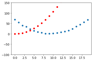
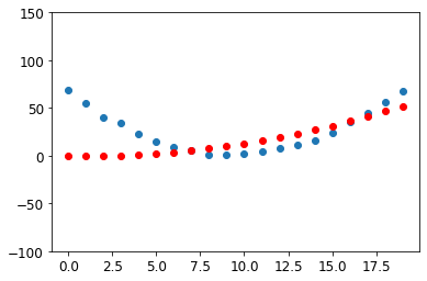
First fit with the actual data in blue and the fitted model in red.

We want to calculate the gradients of the parameters, and then adjust the parameters by some small fraction of those gradients. Taking small steps allows for incremental improvements in the parameters and avoids divergence.

In this case we will iterate through the process 25 times. 25 times is an arbitrary choice and in practice observation of the loss would help indicate when to stop.

# Create function to run through this process on repeat

def apply_step(params, prn=True):
    preds = f(time, params)
    loss = mse(preds, speed)
    loss.backward()
    params.data -= lr * params.grad.data
    params.grad = None
    if prn: print(loss.item())
    return preds

# Repeat it 25 times, outputting the loss

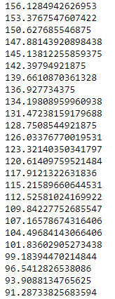
for i in range(25): apply_step(params)
The output of our arbitrary 25 iterations

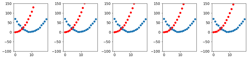
A plot of the first few graphs shows small changes to the model each time, as it moves slowly towards a better fit.

And here is the plot after 100 iterations.

More resources:
Builtin.com
3Blue1Brown on Youtube

Guinness Image Classifier: Training the model in Python using fastai

I have been learning about Neural Networks and Image Classifiers through fastai recently, and wanted to try apply what I had learned to a problem outside the scope of that material.

The Problem

Any Irish person that drinks Guinness will probably have strong opinions on the quality of the drink in just about any pub they’ve been in (and non-Guinness drinkers might claim that it is all nonsense). The opinions range from ‘beautiful’ to slightly more offensive at the other end of the scale. Recently social media has filled with examples of lovingly-crafted and not-so-lovingly-crafted beverages.

I wanted to train a Neural Network to be able to distinguish between a good and a bad pint, and have documented the process of training the model below.

The Data

I collected approximately 300 images of pints of Guinness. Sourcing these images from social media helped because they were pre-identified as good or bad pints, making the labelling process easier. I didn’t do any cleaning on the images before trying to train the model – instead after training I used fastai’s built-in cleaning functionality to easily identify images that were not appropriate for the model.

The process to scrape and organise the images will become a post of its own at some point.

Examining the Data

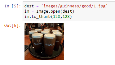
Checking a single image, to make sure file path works and that the filetype is actually an image.

Image 1 in the ‘good pints’ dataset.

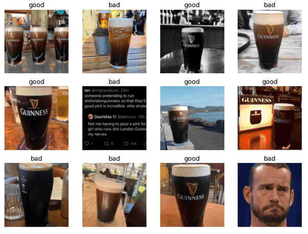
Pulling a set of images in, with their labels. Here we see that a few of the images are not pictures of pints, and these will need to be cleaned. fastai makes identifying them and deleting them fairly convenient, and will happen after the first round of model training.

Some good pints, some bad pints, and some non-pints.

Model Training Attempt 1

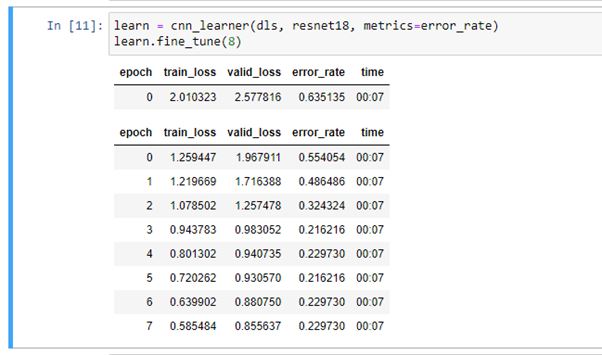
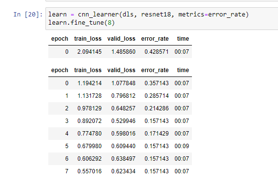
Without further ado, we get into it. Below is the first output of the model fitting. The neural network applies transfer learning based on fastai’s resnet18, over 8 epochs. Loss rates on the training and validation datasets decrease fairly steadily, while the classification error rate levels off after 4 or 5 epochs.

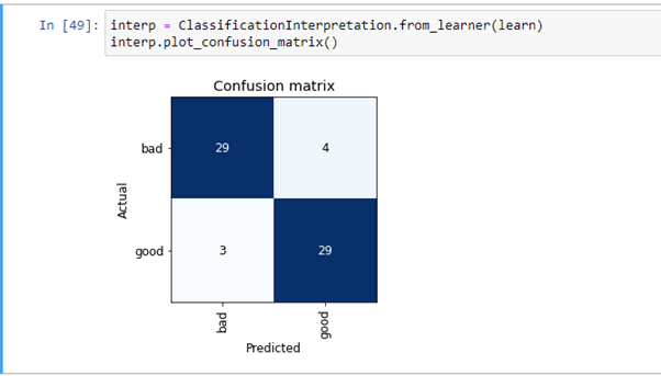
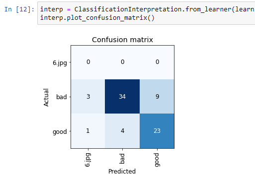
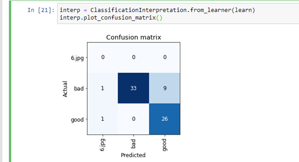
And the confusion matrix gives us a visual depiction of how the validation date is classified. It also tells us whether bad pints are being misclassified as good or vice-versa. The first thing I learned here is that there is something off with the data structures that I am feeding into the model. As well as good and bad, the matrix has a category of ‘6.jpg’ which obviously shouldn’t be there. ‘number.jpg’ is the format I would expect from the images I am using, so something has gone wrong there. Apart from that things don’t look too terrible. This iteration of the model classified 9 good pints as bad, and 4 bad pints as good.

Confusion Matrix for the first model training attempt.

Data Clean 1

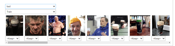
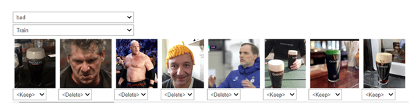
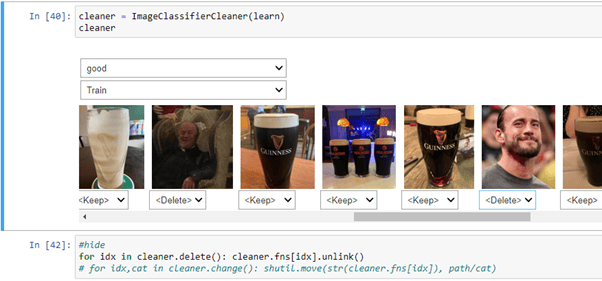
Fastai’s functionality for cleaning images displays the images that the model is least sure about, and then allows the user to make quick decisions on deleting or recategorising them. You can do this across the training and validation set, and the categories within the data (in this case ‘good’ and ‘bad’).

Here’s how that looks. Clearly there are some odd images in here.

Before making cleaning decisions.
After making cleaning decisions. Delete delete delete.

I applied the same process to the ‘bad’ validation set, and both datasets for the ‘good’ group.

Model Training Attempt 2 + 3

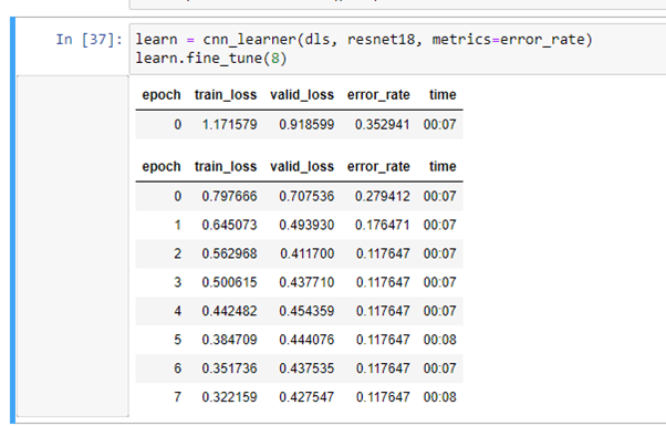
Immediately the results are better.

Attempt 2
Attempt 2

Oops. Still hadn’t fixed that ‘6.jpg’. A quick check of the data showed that there was a folder in with the source images called ‘6.jpg’. This folder was being picked up as a category (with a single image in it), so I corrected that.

Another couple of cleans of the data gives incrementally better results:

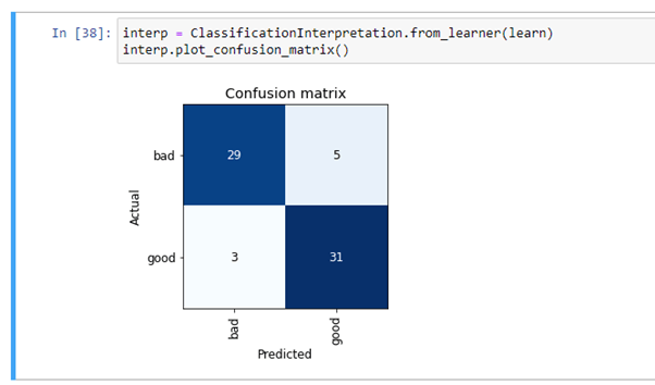
And a classification matrix that actually makes sense.

But there is still some image cleaning to be done:

The final (for now) model

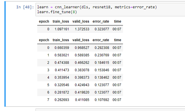
After a final clean, the last run of the model gives us slightly better results again, with an error rate of just over 10%.

The final results from the model.

And the classification matrix shows 58 correct classifications, with 7 incorrect classifications.

The final classification matrix.

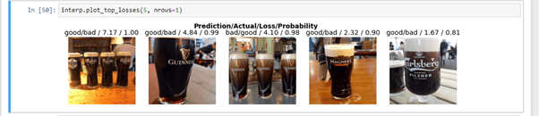
Here are some of the image that the model is classifying incorrectly. The tags above the images show prediction/actual, so good/bad means the model thought it was good and that it was actually bad. The final figure identifies the probability the model assigned to it – aka how confident the model was.
The images that confused the mode are interesting. It doesn’t seem to do well with images of multiple pints. Also, the first image shows pints that look decent in a non-Guinness glass. Feeding the model a lot more data might allow it to learn to differentiate between glass types or brand logos.

These confused the model. I’m a bit confused myself.

What next?

I exported the model and will publish it using Binder. I’ll also try set up an embedded model in this blog.

Finally, I’ll look at what improvements I can make to the model to improve its accuracy.

The code is on github.