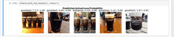
neural networks – Yet Another Data Analytics Blog

Cross Entropy Loss

In a previous blog post I described the process of training a neural network for classifying the quality of Guinness. That was a binary classification problem (the result was ‘good’ or ‘bad’) and a key step in it was using the sigmoid function to ensure that the model’s activations were between 0 and 1. This blog post looks at the methods used for classification with neural net loss functions in binary and multi-class scenarios.

To make the scenarios easier to work through, I will use simple numerical examples where possible.

The Binary Case

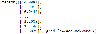
Consider a neural net that has to classify into two categories – identifying an image as a cat or a dog. The way the classification works in practice is this – with 6 images that are run through our model, and we get a single activation score out for each image:

torch.random.manual_seed(42);

acts = torch.randn((6,1))*2
acts

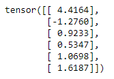
These activation scores aren’t automatically interpretable, and the values don’t have a relatable meaning. To help with this, they are fed through the sigmoid function. The sigmoid function translates any value to a value between 0 and 1. This means our activations have an interpretable, common scale, and they can be considered synonymous with probabilities.

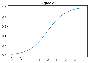
After our activation scores are fed through the sigmoid function we get:

acts.sigmoid()

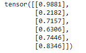
Output of the sigmoid function are always between 0 and 1.

We can consider these activations as probabilities that the input image is classified as one of our binary categories. For example, if the model is categorising cats and dogs, then our model is 98.81% sure that the first image is a cat, and 21.82% sure that the second image is a cat (which means it is 78.18% sure that it is a dog).

The actual measure of loss depends on whether the model is correct or not. In the example above, if the first image is a cat, then the loss is (1-0.9881). If the first image is a dog, then the loss is 0.9881. The benefit of this approach is that the loss is dependent on the model’s confidence in its classifications, not the amount of classifications it gets correct or incorrect. This means a small change of parameters (e.g. from Gradient Descent) will always cause a change in loss, even if the classification decision has not changed.

Another approach to the Binary case

Here’s another way of looking at the binary case: what if we create two activations, one for the ‘cat’ and one for the ‘dog’?

acts = torch.randn((6,2))*2
acts

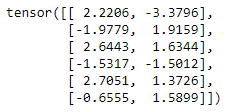
So here we have two activations for each image – one for the ‘cat’ and one for the ‘dog’. One of the complexities this introduces is that these activations are independent from eachother. In the first row above, 2.2206 and -3.3796 are not directly dependent on eachother. This means that when the activations are fed through the sigma function the probabilities don’t really make sense. The probabilities in the rows below don’t sum to 1 as we would expect them to.

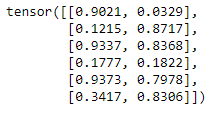
Outputs of the sigmoid function don’t really make sense as probabilities here.

What’s happening is that we are not really getting a true probability. We getting the model’s confidence in relation to each category. Whether the numbers are high or low doesn’t matter, what matters is which is higher or lower in comparison to the other.

To convert this into something that we can solve with the sigmoid function we do the following: get the difference between the activations and put that through the sigmoid function. The difference between the activations represents how much more sure the model is about category A vs B, or cat vs dog.

(acts[:,0]-acts[:,1]).sigmoid()

The sigmoid output of the difference between the activation scores.

This ‘trick’ to utilise the sigmoid with two activation values already has a name – the softmax function.

Softmax

From wikipedia:

The softmax function takes as input a vector z of K real numbers, and normalizes it into a probability distribution consisting of K probabilities proportional to the exponentials of the input numbers. That is, prior to applying softmax, some vector components could be negative, or greater than one; and might not sum to 1; but after applying softmax, each component will be in the interval {\displaystyle [0,1]} $[0,1]$ , and the components will add up to 1, so that they can be interpreted as probabilities. Furthermore, the larger input components will correspond to larger probabilities.
https://en.wikipedia.org/wiki/Softmax_function

And in function form:

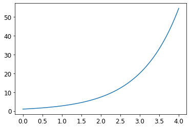
In short, the function takes a list of real numbers, and transforms them into a set of probabilities. It can take negative numbers as input. The output will always sum to 1. This works because the exponential function always outputs a positive number. Using the exponential function also means that inputs that are slightly larger will be assigned much larger probabilities. For example exp(4) = 55 and exp(8) = 2981. This means the softmax is likely to assign a single category as the definitive ‘winner’ – which is helpful for training.

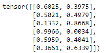
Applying this to our example gives the same result that the alternative application of the sigmoid function did!

sm_acts = torch.softmax(acts, dim=1)
sm_acts

The second part of cross entropy loss is the log likelihood.

Log Likelihood

We could calculate Loss directly from the softmax output above. To do this we would compare our labels to the probabilities assigned, and pull the values from the softmax output based on the labels. For example, if the first column represents the probability that the image is a cat, and we know that the first image is a cat, then we’d take the 0.6025. If the label for the second row indicates that it’s a dog, then we’d take 0.8668, and so on. This generalises nicely to a situation with three, ten or a hundred categories.

One shortfall of this is that the loss is then being expressed using probabilities. This means that the model would think of 0.99 and 0.999 as very similar, when in reality 0.99 is incorrect 1/100 times, and 0.999 is incorrect 1/1000 times, and that might be a massive difference in accuracy for a particular problem.

The solution to this is to run these values through the log function. The log function will convert the probabilities (range 0:1) to a log scale with range (-infinity: 0). Then it takes the negative value of that. So a correct classification with a high probability gets a value close to 0, and an incorrect classification with a high probability gets a very large value. Since the aim is to minimise loss, this penalises the model for incorrect classifications,

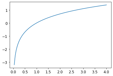
Natural log from 0 to 4. All probabilities will fall in the range of 0-1, and will get values assigned from -inf to 0.

All these transformations are neatly named the Negative Log Likehood. In practice then we get the softmax, calculate its log, and calculate the negative log likelihood based on that. This is Cross Entropy Loss! PyTorch does that in the following function:

loss_func = nn.CrossEntropyLoss()

loss_func(acts, targ)

This give our example an output of 1.8045. We can also split that loss value out into the individual values for each row:

nn.CrossEntropyLoss(reduction='none')(acts, targ)

1.8045 is just the mean of these values.

All-in-all this functions as an effective loss function because:
1. It works for multi-category problems
2. Softmax produces probabalistic activations
3. Softmax wants to pick a winning categorisation
4. The log functions allows for differentiation of small probability differences

Final benefit of Logs

One final note on the benefit of logs:

Log(a x b) = Log(a) + Log(b)

This simple expression is very useful when dealing with very small and very large numbers. Being able to replace multiplication with addition reduces risk of computational inaccuracies from floating point errors. Computers are then a lot less likely to end up with scales of numbers that they can’t handle.

Building a Neural Network from scratch using PyTorch and FastAI

This post follows content from fastai to build a two layer Neural Network from scratch using python. The code is saved on my github.

The data, and data prep

I used a sample dataset from FastAI based on a famous computer vision dataset, MNIST. The sample dataset uses 3s and 7s only, to make the overall problem simpler.

After importing the required packages and connecting to the data, we can see some of the images in the dataset. There are over 6000 ‘3s’ in the dataset. Here are a few of them:

They can also be viewed as arrays, where each pixel has a value between 0 (white) and 255 (black). This is the top portion of one.

It is easier to see if the array is shaded.

Using python we can stack the images into a single tensor, and then see what the ‘average’ 3 or 7 looks like:

# creating lists of the images in the 7 and 3 folders
seven_tensors = [tensor(Image.open(o)) for o in sevens]
three_tensors = [tensor(Image.open(o)) for o in threes]
len(three_tensors),len(seven_tensors)
# using torch.stack to stack the tensors into a 3 dimensional tensor
stacked_sevens = torch.stack(seven_tensors).float()/255
stacked_threes = torch.stack(three_tensors).float()/255
stacked_threes.shape
# the average 3
mean3 = stacked_threes.mean(0)
show_image(mean3);
# the average 7
mean7 = stacked_sevens.mean(0)
show_image(mean7);

Structuring the data for the Neural Net

Using PyTorch we get the data into a format and shape that works for our calculations. Our images are transformed into a tensor with 12396 rows and 784 columns. The 784 columns represent the 28 x 28 pixels, flattened. Our labels are a vector with 12396 rows and 1 column.

train_x = torch.cat([stacked_threes, stacked_sevens]).view(-1, 28*28)
train_y = tensor([1]*len(threes) + [0]*len(sevens)).unsqueeze(1)
train_x.shape,train_y.shape

The data in the correct shape and format.

The training data is put into a dataset where the x,y variables are available as a tuple. x is the 784 pixels of an image and y is the label. The same prep is applied to the validation data.

dset = list(zip(train_x,train_y))
x,y = dset[0]
x.shape,y

The prepared dataset, in tuple form.

With a set of randomly generated weights and biases, a simple linear model of the form y = ax + b is created, and when the training data is applied to it, a score for every image is output:

def linear1(xb): return xb@weights + bias
preds = linear1(train_x)
preds

Turns out this has a 57% accuracy, so not much better than guessing. This is to be expected since the weights were randomly generated.

The next step should be to update the weights in a way that improves the accuracy slightly. One issue with this is that a small change in the weights might not change the accuracy at all, causing the algorithm to get stuck. Introducing the sigmoid function; It is a smooth continuous function that will always give a different output for small changes in weights. This allows us to make and measure the effect of small changes in the parameters, so that the model moves in the right direction.
Any input to the function always gives an output between 0 and 1.

Putting the model together

All in all then, we do the following:
1. Initialise a set of random weights and biases
2. Apply our training data to the model
3. Calculate the loss of the predictions compared to the correct answers
4. Calculated the gradients of the parameters and adjust the parameters
5. Go back to step 2

# This function:
#     Takes the input data
#     Makes predictions based on the model ax + b
#     Calculates the loss using the sigmoid functionality when comparing to the dependent values
#     Calculated the gradients using the .backward() method
def calc_grad(xb, yb, model):
    preds = model(xb)
    loss = mnist_loss(preds, yb)
    loss.backward()
def train_epoch(model, lr, params):
    for xb,yb in dl:
        calc_grad(xb, yb, model)
        for p in params:
            p.data -= p.grad*lr
            p.grad.zero_()
def batch_accuracy(xb, yb):
    preds = xb.sigmoid()
    correct = (preds>0.5) == yb
    return correct.float().mean()
def validate_epoch(model):
    accs = [batch_accuracy(model(xb), yb) for xb,yb in valid_dl]
    return round(torch.stack(accs).mean().item(), 4)

Running the code for 20 epochs shows increasing accuracy

for i in range(20):
    train_epoch(linear1, lr, params)
    print(validate_epoch(linear1), end=' ')

Accuracy after each epoch.

Adding Nonlinearity

Adding a nonlinear layer gives us a true neural net. Here is a tw0-layer neural net, with a RELU layer in between.

def simple_net(xb): 
    res = xb@w1 + b1
    res = res.max(tensor(0.0))
    res = res@w2 + b2
    return res

Here’s the nonlinear aspect introduced by the RELU function, visualised:

Much of this can be replaced with ready-made components from either PyTorch or fastai, making it easier to implement,

simple_net = nn.Sequential(
    nn.Linear(28*28,30),
    nn.ReLU(),
    nn.Linear(30,1)
)
learn = Learner(dls, simple_net, opt_func=SGD,
                loss_func=mnist_loss, metrics=batch_accuracy)
learn.fit(40, 0.1)

The accuracy after 40 epochs is 98.2%. A quick comparison with more mature methods shows that there is still lots more to do: a single epoch of fastai’s resnet18 model gives accuracy of 99.7%!

dls = ImageDataLoaders.from_folder(path)
learn = cnn_learner(dls, resnet18, pretrained=False,
                    loss_func=F.cross_entropy, metrics=accuracy)
learn.fit_one_cycle(1, 0.1)

Output from one epoch of Resnet18

Guinness Image Classifier: Training the model in Python using fastai

I have been learning about Neural Networks and Image Classifiers through fastai recently, and wanted to try apply what I had learned to a problem outside the scope of that material.

The Problem

Any Irish person that drinks Guinness will probably have strong opinions on the quality of the drink in just about any pub they’ve been in (and non-Guinness drinkers might claim that it is all nonsense). The opinions range from ‘beautiful’ to slightly more offensive at the other end of the scale. Recently social media has filled with examples of lovingly-crafted and not-so-lovingly-crafted beverages.

I wanted to train a Neural Network to be able to distinguish between a good and a bad pint, and have documented the process of training the model below.

The Data

I collected approximately 300 images of pints of Guinness. Sourcing these images from social media helped because they were pre-identified as good or bad pints, making the labelling process easier. I didn’t do any cleaning on the images before trying to train the model – instead after training I used fastai’s built-in cleaning functionality to easily identify images that were not appropriate for the model.

The process to scrape and organise the images will become a post of its own at some point.

Examining the Data

Checking a single image, to make sure file path works and that the filetype is actually an image.

Pulling a set of images in, with their labels. Here we see that a few of the images are not pictures of pints, and these will need to be cleaned. fastai makes identifying them and deleting them fairly convenient, and will happen after the first round of model training.

Some good pints, some bad pints, and some non-pints.

Model Training Attempt 1

Without further ado, we get into it. Below is the first output of the model fitting. The neural network applies transfer learning based on fastai’s resnet18, over 8 epochs. Loss rates on the training and validation datasets decrease fairly steadily, while the classification error rate levels off after 4 or 5 epochs.

And the confusion matrix gives us a visual depiction of how the validation date is classified. It also tells us whether bad pints are being misclassified as good or vice-versa. The first thing I learned here is that there is something off with the data structures that I am feeding into the model. As well as good and bad, the matrix has a category of ‘6.jpg’ which obviously shouldn’t be there. ‘number.jpg’ is the format I would expect from the images I am using, so something has gone wrong there. Apart from that things don’t look too terrible. This iteration of the model classified 9 good pints as bad, and 4 bad pints as good.

Confusion Matrix for the first model training attempt.

Data Clean 1

Fastai’s functionality for cleaning images displays the images that the model is least sure about, and then allows the user to make quick decisions on deleting or recategorising them. You can do this across the training and validation set, and the categories within the data (in this case ‘good’ and ‘bad’).

Here’s how that looks. Clearly there are some odd images in here.

After making cleaning decisions. Delete delete delete.

I applied the same process to the ‘bad’ validation set, and both datasets for the ‘good’ group.

Model Training Attempt 2 + 3

Immediately the results are better.

Oops. Still hadn’t fixed that ‘6.jpg’. A quick check of the data showed that there was a folder in with the source images called ‘6.jpg’. This folder was being picked up as a category (with a single image in it), so I corrected that.

Another couple of cleans of the data gives incrementally better results:

And a classification matrix that actually makes sense.

But there is still some image cleaning to be done:

The final (for now) model

After a final clean, the last run of the model gives us slightly better results again, with an error rate of just over 10%.

And the classification matrix shows 58 correct classifications, with 7 incorrect classifications.

Here are some of the image that the model is classifying incorrectly. The tags above the images show prediction/actual, so good/bad means the model thought it was good and that it was actually bad. The final figure identifies the probability the model assigned to it – aka how confident the model was.
The images that confused the mode are interesting. It doesn’t seem to do well with images of multiple pints. Also, the first image shows pints that look decent in a non-Guinness glass. Feeding the model a lot more data might allow it to learn to differentiate between glass types or brand logos.

These confused the model. I’m a bit confused myself.

What next?

I exported the model and will publish it using Binder. I’ll also try set up an embedded model in this blog.

Finally, I’ll look at what improvements I can make to the model to improve its accuracy.

The code is on github.