This post looks at the concept of gradient descent, and applies it to a simple function. It is prompted by and takes some code from the fastai lesson content.
Put simply, gradient descent is used to give feedback to a deep learning model so it can adjust its parameters. The intention is to prompt the model to adjust the parameters so that the model will improve slightly, and make repeated improvements so that the model gets iteratively better.
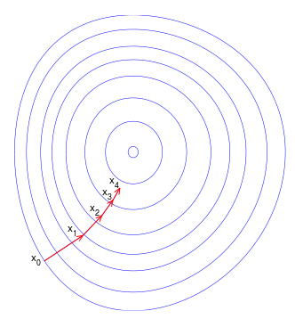
Mathematically, it is an algorithm for finding the local minimum of a differentiable function. The differentiable function in this case is the loss function of the model, and the local minimum represents the (or one of the) best set(s) of parameters for the model.
The full code for this is saved here. I’ll include highlights and graphs in this post.
First, we generate a simple dataset to train our model to.
# Define a tensor of time values
time = torch.arange(0,20).float(); time
# Define a tensor of speed values, with a quadratic element built in
speed = torch.randn(20)*2 + 0.75*(time-9.5)**2 + 1
plt.scatter(time,speed);
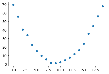
Then, define a function as the basis for our model (in this case it is a quadratic function), and a loss function (mean square error).
# We base our model on a quadratic function, based on the shape of the plot
# Need to solve for a, b and c

def f(t, params):
    a,b,c = params
    return a*(t**2) + (b*t) + c

# Also define a function to measure loss. The mean squared error works.

def mse(preds, targets): return ((preds-targets)**2).mean().sqrt()
Initialising the parameters, making the predictions, and plotting them:
params = torch.randn(3).requires_grad_()
orig_params = params.clone()

preds = f(time, params)
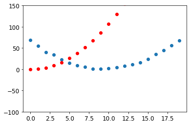
We want to calculate the gradients of the parameters, and then adjust the parameters by some small fraction of those gradients. Taking small steps allows for incremental improvements in the parameters and avoids divergence.
In this case we will iterate through the process 25 times. 25 times is an arbitrary choice and in practice observation of the loss would help indicate when to stop.
# Create function to run through this process on repeat

def apply_step(params, prn=True):
    preds = f(time, params)
    loss = mse(preds, speed)
    loss.backward()
    params.data -= lr * params.grad.data
    params.grad = None
    if prn: print(loss.item())
    return preds

# Repeat it 25 times, outputting the loss

for i in range(25): apply_step(params)
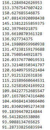
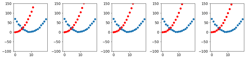
A plot of the first few graphs shows small changes to the model each time, as it moves slowly towards a better fit.
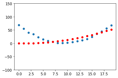
And here is the plot after 100 iterations.
More resources:
Builtin.com
3Blue1Brown on Youtube

