Classifying Pet Breeds and Fine-Tuning a Neural Net

This post follows fastai’s content on building, training and fine-tuning Neural Networks. It leverages one of the examples provided in their course involving classifying the breeds of dogs and cats.

The code for this example is stored on my GitHub.

Connecting to the data and pre-sizing the images

I connected to fastai’s PETS dataset, and used regex to extract the label names from the file names.
Full details on the Oxford-IIIT Pet dataset here.

Some of the code applied, using fastai’s DataBlock:

pets = DataBlock(blocks = (ImageBlock, CategoryBlock),
#                  telling the DataBlock that the data is image based
                 get_items=get_image_files, 
#                  set random seed
                 splitter=RandomSplitter(seed=42),
#                  use regex to extract y values from names
                 get_y=using_attr(RegexLabeller(r'(.+)_\d+.jpg$'), 'name'),
#                  resize and transfom as part of presizing
                 item_tfms=Resize(460),
                 batch_tfms=aug_transforms(size=224, min_scale=0.75))

# pointing the DataBlock to the images directory
dls = pets.dataloaders(path/"images")

One of the lines above (item_tfms=Resize(460)) pre-sizes the images.

Pre-sizing is image preprocessing that does several things: give images same dimensions, so they can be transformed to tensors for GPU-based operations. Keeping image sizes consistent reduces the amount of distinct augmentation computations that are required, and makes for more efficient processing

Many common data augmentation transforms introduce spurious empty patches or degrade data. For example, simple rotation will introduce empty pixels into the image. Other techniques may interpolate pixels.

The solution works in two steps:

  1. Resize to a fairly large size, so all images are consistent.
  2. Combine the individual augmentations into one and perform the combined operation on the GPU once, instead of performing operations individually.

The resize creates images large enough to leave margins for further augmentation.

The GPU is used for all data augmentation, and all operations are done together, with a single interpolation at the end.

The fastai course content shows an interesting comparison between their pre-sizing operations (left) and the same transformations applied with a more traditional approach (right).
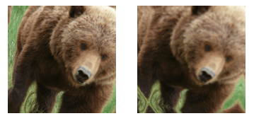
Image from fastai’s course documentation.


Here are a few examples from the datablock, to make sure the data is loaded correctly.

A few examples of the loaded and prepared images

Fastai often recommends training to a simple model initially, rather than overengineering an elaborate model from the start. This helps establish a baseline and gives an idea of the data can train a model at all.

Below, applying the loaded data to a neural net, with error rate used as the metric, and resnet34 used for transfer learning.

learn = cnn_learner(dls, resnet34, metrics=error_rate)
learn.fine_tune(2)
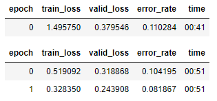
A baseline run.

That loss is the function chosen to optimize the parameters of the model. Fastai tries to select an appropriate loss function based on what kind of data and model being used. In this case, with image data and a categorical outcome, fastai defaults to using cross-entropy loss.

Cross-entropy loss is a loss function works efficiently with multiple categories. I have already written a blog post on it, here: https://frankiecoughlan.data.blog/2021/12/10/cross-entropy-loss/

Model Interpretation

A confusion matrix will help see where the model is doing well, and where it’s doing badly:

interp = ClassificationInterpretation.from_learner(learn)
interp.plot_confusion_matrix(figsize=(12,12), dpi=60)
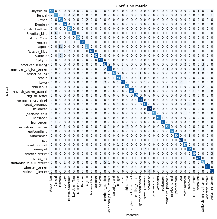
The confusion matrix with 37 categories.

That confusion matrix is a little awkward to read. The most_confused method will show the cells of the confusion matrix with the most incorrect predictions.

interp.most_confused(min_val=5)

The breeds that the model got most confused over.

Taking this as the baseline, the next section focuses on further improvements.

Improving the Model

The Learning Rate Finder

Finding the right learning rate is important:
Too low and it will take a long time to train. This wastes time, but can also cause overfitting.
Too high and it will overstep, overshooting the minimum loss. Repeating that can move the model away from the optimum solution, not closer.

This happens below with a learning rate of 10%

learn = cnn_learner(dls, resnet34, metrics=error_rate)
learn.fine_tune(1, base_lr=0.1)
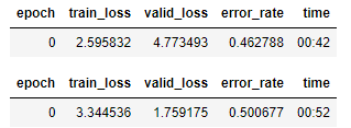
Poor performance with a very high learning rate.

One approach to find the optimum learning rate (from Leslie Smith in 2015) is called the learning rate finder. Start with a tiny learning rate, use it for one mini-batch, and measure the loss. Double the rate, use it for one mini-batch, and measure the loss again. The loss will improve because we’ve taken a slightly bigger step in the right direction. Repeat until the loss gets worse. At that point, the learning rate is too large. It’s common to select a learning rate slightly lower than that which produced the worsening loss. Two recommendations for choosing that point are (a) one order of magnitude lower that that where the minimum loss was achieved, or (b) the last point where the loss was clearly decreasing. (a) and (b) are often very similar.

The default learning rate for fastai is 1e-3.

learn = cnn_learner(dls, resnet34, metrics=error_rate)
lr_steep = learn.lr_find()
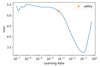
In the graph above, learning rates lower than 1e-4 won’t allow the model to train – the slope is flat.
Rates higher than 1e-1 will cause the model to diverge – positive slope.
The point that produces the minimum loss is tempting, but the slope is flat here too.
The sweet spot is the point in the graph with the steepest negative slope.

learn = cnn_learner(dls, resnet34, metrics=error_rate)
learn.fine_tune(2, base_lr=3e-3)
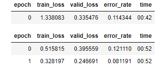
Better performance with a single chosen learning rate.

Unfreezing and Transfer Learning

Transfer learning in a nutshell:

We take a pretrained model that is finetuned for a particular task. It has linear layers, with a nonlinear activation function between each linear pair, and an activation function like softmax at the end. The final linear layer uses a matrix with enough columns that the output size = number of classes in the classification problem.

This final linear won’t help when we are transfer learning, because it is specifically designed to classify the categories in the original context. So when transfer learning that layer is discarded and replaced with a layer that provides the correct number of outputs for the new problem. This new linear layer is random, but the output of the entire model isn’t random because this final random layer sits on top of all the prior carefully trained layers.

The aim is to retain all the useful things learned in early layers and then apply them to our new problem. The trick is to freeze the weights for the prior layers, and tell the optimizer to only update the weights in the later randomly added layers.

Fastai automatically freezes pretrained layers when creating a model from a pretrained network. The fine_tune method makes fastai do two things:
Train the randomly added layers for one epoch, with all other layers frozen
Unfreeze all the layers, and train them for all the epochs required

The method has parameters that can change its behaviour, or we can call the underlying methods directly to get custom behaviour. fit_one_cycle is fastai’s method for training without fine_tune.

learn = cnn_learner(dls, resnet34, metrics=error_rate)
learn.fit_one_cycle(3, 3e-3)

Then we’ll unfreeze the model, and run lr_find again, because having more layers to train, and weights that have already been trained for three epochs, means our previously found learning rate isn’t appropriate any more.
The graph looks different this time – the flat line followed by the sharp increase is due to the fact that the model has been trained already. Looking for the point with maximum gradient won’t help here, and instead it makes sense to choose a point well before the sharp increase, like 1e-5.
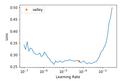
The learning rate finder on a transfer-learning model.

Training at that learning rate improved the model a bit, but there’s more that can be done.
Discriminative Learning Rates

After unfreezing, all of the weights can be changed by further training. However the quality or usefulness of the pretrained weights is higher than that of the randomly added parameters. The pretrained weights have been trained over a high number of epochs with a lot of data. The implication is that those pretrained weights would be better off with a lower learning rate, since less drastic change is required.

Also, earlier layers typically have learned generally useful things – like detecting edges and gradients – which is useful for any task. Later layers are far more specific, and so may be less relevant to the new task. It seems reasonable to let the later layers fine tune more quickly than the earlier ones.

Fastai’s default approach is to use discriminative learning rates. It uses lower learning rates in the early layers and higher learning rate for the later layers.

In Fastai you can pass a first and last learning rate to the model (via a python slice object) and it will start training with the first rate, and finish with the last rate, making incremental steps in between.

See below for previous training reapplied with discriminative learning rates.

learn = cnn_learner(dls, resnet34, metrics=error_rate)
learn.fit_one_cycle(3, 3e-3)
learn.unfreeze()
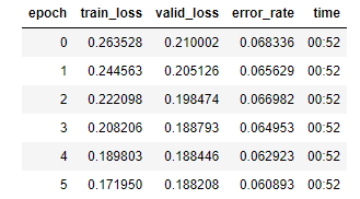
learn.fit_one_cycle(12, lr_max=slice(1e-6,1e-4))
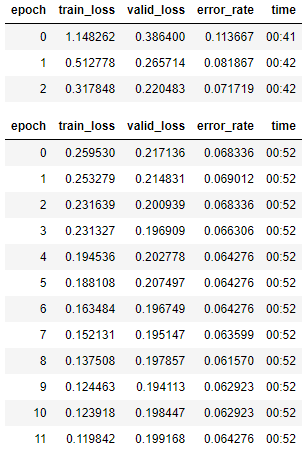
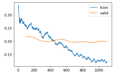
Comparing training loss to validation loss.

The training loss inmproves throughout, but the validation loss slows and plateaus. This is indicating the model is starting to overfit, and becoming overconfident in its predictions.

That doesn’t mean it’s getting less accurate. Accuracy continues to improve even as validation loss gets worse. The end goal is optimising the chosen metrics, not necessarily the loss.

Number of Epochs

If time is a limiting factor, then an initial approach could be to train for the number of epochs that you’re willing to wait for. Then looking at the training/validation loss plots and the metrics will help. If they are still improving in the final epochs then it might be worth training for longer.

If the validation loss get worse towards the end of training, then the model is first getting overconfident, then incorrectly memorizing the data. The latter is the real issue. If the validation loss is deteriorating while the other metrics are improving, then the model can still be performing better.

It’s tempting to run the model for 100 epochs, choose the epoch with the best metrics, and pick that model as the winner. However, this approach doesn’t allow the model to use the smallest rates on the epochs with the best metrics, so the model can’t really fine-tune around the correct area. A better approach is to retrain the model from scratch with the number of epochs adjusted based on where the results were previously good.

Deeper Architectures

In general (but this is a big generalisation), more parameters will lead to more accurate results. Deeper models also use more memory, so deeper models should use smaller batch sizxes to avoid ‘out of memory’ issues on the GPU. Training on deeper architectures can be sped up by using ‘mixed-precision training’, where floating points are reduced from 32 to 16 places where possible.

Trying a deeper architecture with mixed precision:

from fastai.callback.fp16 import *
learn = cnn_learner(dls, resnet50, metrics=error_rate).to_fp16()
learn.fine_tune(6, freeze_epochs=3)
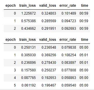
Results from a deeper architecture.

In this case the deeper model doesn’t provide a massive improvement, but the runtime for each epoch has gone from 50 seconds to 5 minutes.
Cross Entropy Loss

In a previous blog post I described the process of training a neural network for classifying the quality of Guinness. That was a binary classification problem (the result was ‘good’ or ‘bad’) and a key step in it was using the sigmoid function to ensure that the model’s activations were between 0 and 1. This blog post looks at the methods used for classification with neural net loss functions in binary and multi-class scenarios.

To make the scenarios easier to work through, I will use simple numerical examples where possible.

The Binary Case

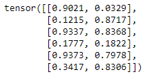
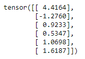
Consider a neural net that has to classify into two categories – identifying an image as a cat or a dog. The way the classification works in practice is this – with 6 images that are run through our model, and we get a single activation score out for each image:

torch.random.manual_seed(42);

acts = torch.randn((6,1))*2
acts
Our activation scores.

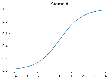
These activation scores aren’t automatically interpretable, and the values don’t have a relatable meaning. To help with this, they are fed through the sigmoid function. The sigmoid function translates any value to a value between 0 and 1. This means our activations have an interpretable, common scale, and they can be considered synonymous with probabilities.

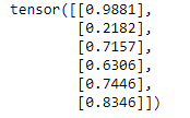
After our activation scores are fed through the sigmoid function we get:

acts.sigmoid()
Output of the sigmoid function are always between 0 and 1.

We can consider these activations as probabilities that the input image is classified as one of our binary categories. For example, if the model is categorising cats and dogs, then our model is 98.81% sure that the first image is a cat, and 21.82% sure that the second image is a cat (which means it is 78.18% sure that it is a dog).

The actual measure of loss depends on whether the model is correct or not. In the example above, if the first image is a cat, then the loss is (1-0.9881). If the first image is a dog, then the loss is 0.9881. The benefit of this approach is that the loss is dependent on the model’s confidence in its classifications, not the amount of classifications it gets correct or incorrect. This means a small change of parameters (e.g. from Gradient Descent) will always cause a change in loss, even if the classification decision has not changed.

Another approach to the Binary case

Here’s another way of looking at the binary case: what if we create two activations, one for the ‘cat’ and one for the ‘dog’?

acts = torch.randn((6,2))*2
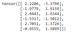
acts
Two activations for the binary case.

So here we have two activations for each image – one for the ‘cat’ and one for the ‘dog’. One of the complexities this introduces is that these activations are independent from eachother. In the first row above, 2.2206 and -3.3796 are not directly dependent on eachother. This means that when the activations are fed through the sigma function the probabilities don’t really make sense. The probabilities in the rows below don’t sum to 1 as we would expect them to.

Outputs of the sigmoid function don’t really make sense as probabilities here.

What’s happening is that we are not really getting a true probability. We getting the model’s confidence in relation to each category. Whether the numbers are high or low doesn’t matter, what matters is which is higher or lower in comparison to the other.

To convert this into something that we can solve with the sigmoid function we do the following: get the difference between the activations and put that through the sigmoid function. The difference between the activations represents how much more sure the model is about category A vs B, or cat vs dog.

(acts[:,0]-acts[:,1]).sigmoid()
The sigmoid output of the difference between the activation scores.

This ‘trick’ to utilise the sigmoid with two activation values already has a name – the softmax function.

Softmax

From wikipedia:

The softmax function takes as input a vector z of K real numbers, and normalizes it into a probability distribution consisting of K probabilities proportional to the exponentials of the input numbers. That is, prior to applying softmax, some vector components could be negative, or greater than one; and might not sum to 1; but after applying softmax, each component will be in the interval {\displaystyle [0,1]}[0,1], and the components will add up to 1, so that they can be interpreted as probabilities. Furthermore, the larger input components will correspond to larger probabilities.

https://en.wikipedia.org/wiki/Softmax_function

And in function form:

The softmax function.

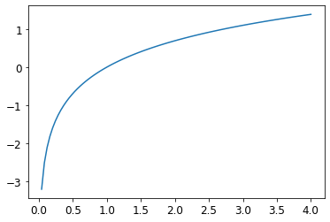
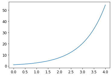
In short, the function takes a list of real numbers, and transforms them into a set of probabilities. It can take negative numbers as input. The output will always sum to 1. This works because the exponential function always outputs a positive number. Using the exponential function also means that inputs that are slightly larger will be assigned much larger probabilities. For example exp(4) = 55 and exp(8) = 2981. This means the softmax is likely to assign a single category as the definitive ‘winner’ – which is helpful for training.

Exponential function from 0 to 4.

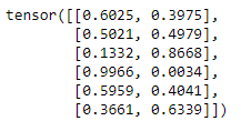
Applying this to our example gives the same result that the alternative application of the sigmoid function did!

sm_acts = torch.softmax(acts, dim=1)
sm_acts
Softmax output.

The second part of cross entropy loss is the log likelihood.

Log Likelihood

We could calculate Loss directly from the softmax output above. To do this we would compare our labels to the probabilities assigned, and pull the values from the softmax output based on the labels. For example, if the first column represents the probability that the image is a cat, and we know that the first image is a cat, then we’d take the 0.6025. If the label for the second row indicates that it’s a dog, then we’d take 0.8668, and so on. This generalises nicely to a situation with three, ten or a hundred categories.

One shortfall of this is that the loss is then being expressed using probabilities. This means that the model would think of 0.99 and 0.999 as very similar, when in reality 0.99 is incorrect 1/100 times, and 0.999 is incorrect 1/1000 times, and that might be a massive difference in accuracy for a particular problem.

The solution to this is to run these values through the log function. The log function will convert the probabilities (range 0:1) to a log scale with range (-infinity: 0). Then it takes the negative value of that. So a correct classification with a high probability gets a value close to 0, and an incorrect classification with a high probability gets a very large value. Since the aim is to minimise loss, this penalises the model for incorrect classifications,

Natural log from 0 to 4. All probabilities will fall in the range of 0-1, and will get values assigned from -inf to 0.

All these transformations are neatly named the Negative Log Likehood. In practice then we get the softmax, calculate its log, and calculate the negative log likelihood based on that. This is Cross Entropy Loss! PyTorch does that in the following function:

loss_func = nn.CrossEntropyLoss()

loss_func(acts, targ)

This give our example an output of 1.8045. We can also split that loss value out into the individual values for each row:

nn.CrossEntropyLoss(reduction='none')(acts, targ)

1.8045 is just the mean of these values.

All-in-all this functions as an effective loss function because:
1. It works for multi-category problems
2. Softmax produces probabalistic activations
3. Softmax wants to pick a winning categorisation
4. The log functions allows for differentiation of small probability differences

Final benefit of Logs

One final note on the benefit of logs:

Log(a x b) = Log(a) + Log(b)

This simple expression is very useful when dealing with very small and very large numbers. Being able to replace multiplication with addition reduces risk of computational inaccuracies from floating point errors. Computers are then a lot less likely to end up with scales of numbers that they can’t handle.

Building a Neural Network from scratch using PyTorch and FastAI

This post follows content from fastai to build a two layer Neural Network from scratch using python. The code is saved on my github.

The data, and data prep

I used a sample dataset from FastAI based on a famous computer vision dataset, MNIST. The sample dataset uses 3s and 7s only, to make the overall problem simpler.

After importing the required packages and connecting to the data, we can see some of the images in the dataset. There are over 6000 ‘3s’ in the dataset. Here are a few of them:

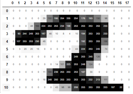
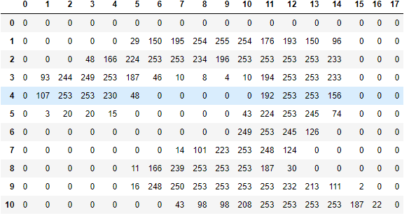
They can also be viewed as arrays, where each pixel has a value between 0 (white) and 255 (black). This is the top portion of one.

It is easier to see if the array is shaded.

Using python we can stack the images into a single tensor, and then see what the ‘average’ 3 or 7 looks like:

# creating lists of the images in the 7 and 3 folders
seven_tensors = [tensor(Image.open(o)) for o in sevens]
three_tensors = [tensor(Image.open(o)) for o in threes]
len(three_tensors),len(seven_tensors)
# using torch.stack to stack the tensors into a 3 dimensional tensor
stacked_sevens = torch.stack(seven_tensors).float()/255
stacked_threes = torch.stack(three_tensors).float()/255
stacked_threes.shape
# the average 3
mean3 = stacked_threes.mean(0)
show_image(mean3);
# the average 7
mean7 = stacked_sevens.mean(0)
show_image(mean7);
The average 3
The average 7.

Structuring the data for the Neural Net

Using PyTorch we get the data into a format and shape that works for our calculations. Our images are transformed into a tensor with 12396 rows and 784 columns. The 784 columns represent the 28 x 28 pixels, flattened. Our labels are a vector with 12396 rows and 1 column.

train_x = torch.cat([stacked_threes, stacked_sevens]).view(-1, 28*28)
train_y = tensor([1]*len(threes) + [0]*len(sevens)).unsqueeze(1)
train_x.shape,train_y.shape
The data in the correct shape and format.

The training data is put into a dataset where the x,y variables are available as a tuple. x is the 784 pixels of an image and y is the label. The same prep is applied to the validation data.

dset = list(zip(train_x,train_y))
x,y = dset[0]
x.shape,y
The prepared dataset, in tuple form.

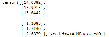
With a set of randomly generated weights and biases, a simple linear model of the form y = ax + b is created, and when the training data is applied to it, a score for every image is output:

def linear1(xb): return xb@weights + bias
preds = linear1(train_x)
preds
The outputted scores.

Turns out this has a 57% accuracy, so not much better than guessing. This is to be expected since the weights were randomly generated.

The next step should be to update the weights in a way that improves the accuracy slightly. One issue with this is that a small change in the weights might not change the accuracy at all, causing the algorithm to get stuck. Introducing the sigmoid function; It is a smooth continuous function that will always give a different output for small changes in weights. This allows us to make and measure the effect of small changes in the parameters, so that the model moves in the right direction.
Any input to the function always gives an output between 0 and 1.

Putting the model together

All in all then, we do the following:
1. Initialise a set of random weights and biases
2. Apply our training data to the model
3. Calculate the loss of the predictions compared to the correct answers
4. Calculated the gradients of the parameters and adjust the parameters
5. Go back to step 2

# This function:
#     Takes the input data
#     Makes predictions based on the model ax + b
#     Calculates the loss using the sigmoid functionality when comparing to the dependent values
#     Calculated the gradients using the .backward() method
def calc_grad(xb, yb, model):
    preds = model(xb)
    loss = mnist_loss(preds, yb)
    loss.backward()
def train_epoch(model, lr, params):
    for xb,yb in dl:
        calc_grad(xb, yb, model)
        for p in params:
            p.data -= p.grad*lr
            p.grad.zero_()
def batch_accuracy(xb, yb):
    preds = xb.sigmoid()
    correct = (preds>0.5) == yb
    return correct.float().mean()
def validate_epoch(model):
    accs = [batch_accuracy(model(xb), yb) for xb,yb in valid_dl]
    return round(torch.stack(accs).mean().item(), 4)

Running the code for 20 epochs shows increasing accuracy

for i in range(20):
    train_epoch(linear1, lr, params)
    print(validate_epoch(linear1), end=' ')
Accuracy after each epoch.

Adding Nonlinearity

Adding a nonlinear layer gives us a true neural net. Here is a tw0-layer neural net, with a RELU layer in between.

def simple_net(xb): 
    res = xb@w1 + b1
    res = res.max(tensor(0.0))
    res = res@w2 + b2
    return res

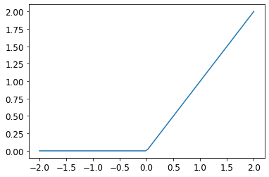
Here’s the nonlinear aspect introduced by the RELU function, visualised:

RELU

Much of this can be replaced with ready-made components from either PyTorch or fastai, making it easier to implement,

simple_net = nn.Sequential(
    nn.Linear(28*28,30),
    nn.ReLU(),
    nn.Linear(30,1)
)
learn = Learner(dls, simple_net, opt_func=SGD,
                loss_func=mnist_loss, metrics=batch_accuracy)
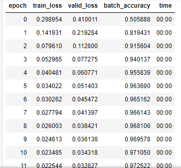
learn.fit(40, 0.1)
Output from the fastai learner.
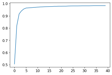
Accuracy, visualised.

The accuracy after 40 epochs is 98.2%. A quick comparison with more mature methods shows that there is still lots more to do: a single epoch of fastai’s resnet18 model gives accuracy of 99.7%!

dls = ImageDataLoaders.from_folder(path)
learn = cnn_learner(dls, resnet18, pretrained=False,
                    loss_func=F.cross_entropy, metrics=accuracy)
learn.fit_one_cycle(1, 0.1)
Output from one epoch of Resnet18

Deploying a Python Neural Net using Binder

The previous blog post trained a neural network to classify images of Guinness. This post will demonstrate how to host the model on Binder so that people can use it themselves.

What is Binder?

The Binder Project helps you create one-click, sharable, live code environments from public code repositories that runs entirely in the cloud. You put your files in a github repository, and point Binder to it. Binder builds a docker image of the repository and hosts it on a JupyterHub server, allowing you to or others to interact with your code in a browser.

Create a github repository and add the required files to it. For this example, I will be adding:
a. A python script that uses widgets to create upload and classify buttons
b. The model trained in the previous post, exported to a .pkl file
c. A requirements text file that specifies the packages that Binder needs

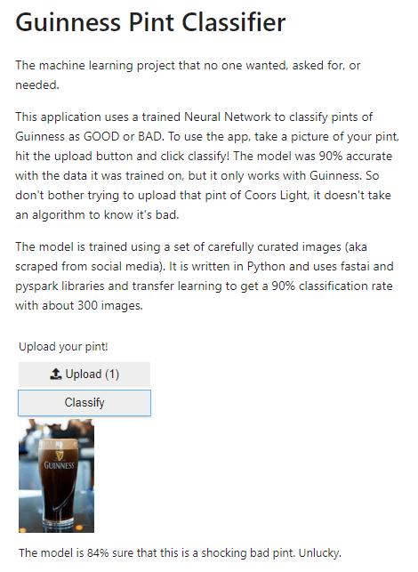
Here is some of the script that will be uploaded. It defines the buttons that will be displayed and the output shown after classification.

# function for image classification
def on_click_classify(change):
    #sets img as an image object based on button upload
    img = PILImage.create(btn_upload.data[-1])
    #clears existing output
    out_pl.clear_output()
    #sets the output as 128x128 and creates a prediction based on learn_inf
    with out_pl: display(img.to_thumb(128,128))
    pred,pred_idx,probs = learn_inf.predict(img)
    if {pred} == 'good':
        lbl_pred.value = f'The model is {probs[pred_idx]:.0%} sure that this is a LOVELY pint. Enjoy!'
    else:
        lbl_pred.value = f'The model is {probs[pred_idx]:.0%} sure that this is a shocking bad pint. Unlucky.'

See the rest of the code at the github repository.

Step 2

Tell Binder where to look! Enter the repository name and a specific file to look for. In this case my file path includes ‘voila/render’ indicating that I want the output to show the widgets and text only – not the code. It gives me a link that I can use to share with others.

This image has an empty alt attribute; its file name is image.png
The Binder Interface.

When I click launch a window opens that establishes the docker image and install the packages in my requirements.txt file. It can take a few minutes to finish.

Step 3

Try it out!

And here is the link to the binder page!