Building a Neural Network from scratch using PyTorch and FastAI

This post follows content from fastai to build a two layer Neural Network from scratch using python. The code is saved on my github.

The data, and data prep

I used a sample dataset from FastAI based on a famous computer vision dataset, MNIST. The sample dataset uses 3s and 7s only, to make the overall problem simpler.

After importing the required packages and connecting to the data, we can see some of the images in the dataset. There are over 6000 ‘3s’ in the dataset. Here are a few of them:

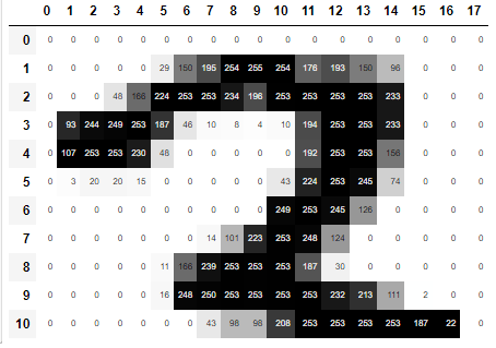
They can also be viewed as arrays, where each pixel has a value between 0 (white) and 255 (black). This is the top portion of one.

It is easier to see if the array is shaded.

Using python we can stack the images into a single tensor, and then see what the ‘average’ 3 or 7 looks like:

# creating lists of the images in the 7 and 3 folders
seven_tensors = [tensor(Image.open(o)) for o in sevens]
three_tensors = [tensor(Image.open(o)) for o in threes]
len(three_tensors),len(seven_tensors)
# using torch.stack to stack the tensors into a 3 dimensional tensor
stacked_sevens = torch.stack(seven_tensors).float()/255
stacked_threes = torch.stack(three_tensors).float()/255
stacked_threes.shape
# the average 3
mean3 = stacked_threes.mean(0)
show_image(mean3);
# the average 7
mean7 = stacked_sevens.mean(0)
show_image(mean7);

Structuring the data for the Neural Net

Using PyTorch we get the data into a format and shape that works for our calculations. Our images are transformed into a tensor with 12396 rows and 784 columns. The 784 columns represent the 28 x 28 pixels, flattened. Our labels are a vector with 12396 rows and 1 column.

train_x = torch.cat([stacked_threes, stacked_sevens]).view(-1, 28*28)
train_y = tensor([1]*len(threes) + [0]*len(sevens)).unsqueeze(1)
train_x.shape,train_y.shape

The training data is put into a dataset where the x,y variables are available as a tuple. x is the 784 pixels of an image and y is the label. The same prep is applied to the validation data.

dset = list(zip(train_x,train_y))
x,y = dset[0]
x.shape,y

With a set of randomly generated weights and biases, a simple linear model of the form y = ax + b is created, and when the training data is applied to it, a score for every image is output:

def linear1(xb): return xb@weights + bias
preds = linear1(train_x)
preds

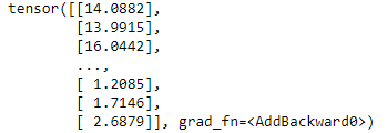
Turns out this has a 57% accuracy, so not much better than guessing. This is to be expected since the weights were randomly generated.

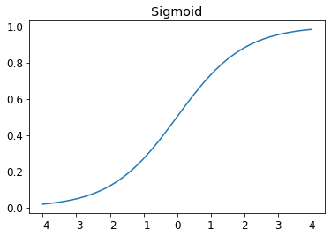
The next step should be to update the weights in a way that improves the accuracy slightly. One issue with this is that a small change in the weights might not change the accuracy at all, causing the algorithm to get stuck. Introducing the sigmoid function; It is a smooth continuous function that will always give a different output for small changes in weights. This allows us to make and measure the effect of small changes in the parameters, so that the model moves in the right direction.
Any input to the function always gives an output between 0 and 1.

Putting the model together

All in all then, we do the following:
1. Initialise a set of random weights and biases
2. Apply our training data to the model
3. Calculate the loss of the predictions compared to the correct answers
4. Calculated the gradients of the parameters and adjust the parameters
5. Go back to step 2

# This function:
#     Takes the input data
#     Makes predictions based on the model ax + b
#     Calculates the loss using the sigmoid functionality when comparing to the dependent values
#     Calculated the gradients using the .backward() method
def calc_grad(xb, yb, model):
    preds = model(xb)
    loss = mnist_loss(preds, yb)
    loss.backward()
def train_epoch(model, lr, params):
    for xb,yb in dl:
        calc_grad(xb, yb, model)
        for p in params:
            p.data -= p.grad*lr
            p.grad.zero_()
def batch_accuracy(xb, yb):
    preds = xb.sigmoid()
    correct = (preds>0.5) == yb
    return correct.float().mean()
def validate_epoch(model):
    accs = [batch_accuracy(model(xb), yb) for xb,yb in valid_dl]
    return round(torch.stack(accs).mean().item(), 4)

Running the code for 20 epochs shows increasing accuracy

for i in range(20):
    train_epoch(linear1, lr, params)
    print(validate_epoch(linear1), end=' ')

Adding Nonlinearity

Adding a nonlinear layer gives us a true neural net. Here is a tw0-layer neural net, with a RELU layer in between.

def simple_net(xb): 
    res = xb@w1 + b1
    res = res.max(tensor(0.0))
    res = res@w2 + b2
    return res

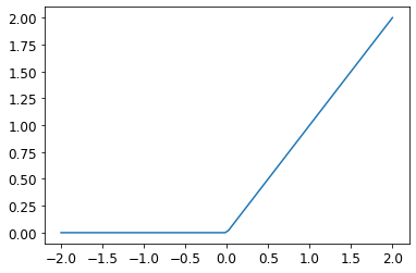
Here’s the nonlinear aspect introduced by the RELU function, visualised:

Much of this can be replaced with ready-made components from either PyTorch or fastai, making it easier to implement,

simple_net = nn.Sequential(
    nn.Linear(28*28,30),
    nn.ReLU(),
    nn.Linear(30,1)
)
learn = Learner(dls, simple_net, opt_func=SGD,
                loss_func=mnist_loss, metrics=batch_accuracy)
learn.fit(40, 0.1)

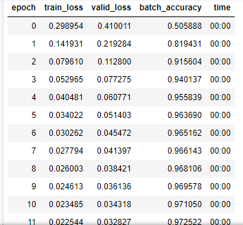
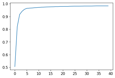
The accuracy after 40 epochs is 98.2%. A quick comparison with more mature methods shows that there is still lots more to do: a single epoch of fastai’s resnet18 model gives accuracy of 99.7%!

dls = ImageDataLoaders.from_folder(path)
learn = cnn_learner(dls, resnet18, pretrained=False,
                    loss_func=F.cross_entropy, metrics=accuracy)
learn.fit_one_cycle(1, 0.1)