Collaborative filtering is a general solution to the following problem: given behavioural features for items, what are the underlying factors that describe or connect them. This sounds very vague, but think of it this way: Netflix uses collaborative filtering to understand the preferences (underlying factors) that its users (items) have, so that it can make recommendations on what to watch.
From Wikipedia:
collaborative filtering is a method of making automatic predictions (filtering) about the interests of a user by collecting preferences or taste information from many users (collaborating). The underlying assumption of the collaborative filtering approach is that if a person A has the same opinion as a person B on an issue, A is more likely to have B’s opinion on a different issue than that of a randomly chosen person.
https://en.wikipedia.org/wiki/Collaborative_filtering
A Simple Dataset
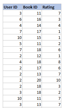
Here’s a portion of a randomly generated dataset containing User IDs, Book IDs, and the users’ book ratings. It’s not in a format that is particularly easy to digest or interpret.
Here’s the same dataset in a format that makes it easier to see patterns within and between users.
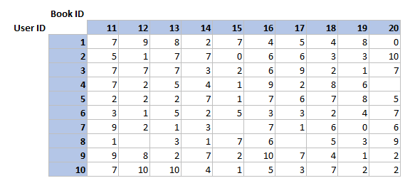
The empty cells in the table above lack ratings. These imply that the user has not read this book. The challenge then, is to understand which books should be recommended to which users, and in what order. If a model can fill the blanks on the table accurately, we can use that to know what books to recommend (or not recommend).
One way to do this is to understand the factors that describe each book and whether the user liked that factor. So if we had information related to genre, writing style and tone and a user’s preference score for each of these factors, then we could derive an overall weighted preference score for the book by multiplying the score.
Assume the scores and factors range from -1 to 1, it might look like this:
Very_like_a_thriller: 0.9
Casual_writing_style: -0.7
Dark_tone: 0.6
A user that loves dark, dense, thrillers might have respective scores of 0.8, -0.7, and 0.8.
Their preference score for this book would be:
0.9×0.8 + (-0.7)x(-0.7) + 0.8×0.6 = 1.69
This calculation is the dot product.
Latent Factors
The underlying factors like genre and tone mentioned above are latent factors. Instead of specifying the latent factors, we can learn them using a general gradient descent approach.
We start by randomly initialising some parameters which represent a set of latent factors for each user. We’ll have to decide how many to use, but for this example I use 3. Each user has a set of factors and each book has a set of factors. In the image below, the latent factors for each user are in yellow and those for each book are in orange. They are random and need to be optimised.
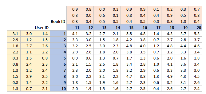
The cells in white above are the predictions, based on the dot product of each user’s factors with each book’s factors. If the prediction is high then it implies the user will like the book, and if it low it implies the user will dislike the book. The max possible score is 10, and the min is 0, to align with the scoring system used in the original dataset.
The next step is to calculate the loss. Mean Squared Error is a good loss function to start with. The MSE for two matrices is calculated as follows:
Get the difference between the actual and predicted values
Square each value
Sum over the matrix
Divide by the number of elements in the matrix
We will move to python and another similar dataset to make this easier to work through.
MovieLens Data and Embeddings
This example uses a dataset called MovieLens. It contains millions of movie rankings. We will use a subset of 100,000 here. The data is available through a fastai function.
from fastai.collab import *
from fastai.tabular.all import *
path = untar_data(URLs.ML_100k)

ratings = pd.read_csv(path/'u.data', delimiter='\t', header=None,
                      names=['user','movie','rating','timestamp'])
ratings.head()
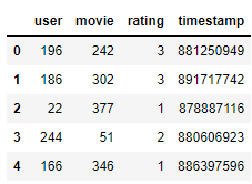
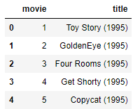
The table u.item contains the mapping of IDs to titles:
movies = pd.read_csv(path/'u.item',  delimiter='|', encoding='latin-1',
                     usecols=(0,1), names=('movie','title'), header=None)
movies.head()
ratings = ratings.merge(movies)
ratings.head()
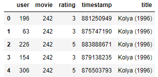
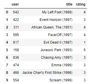
The ratings table contains the data we need to model. We can build a DataLoaders object from it. By default, dataloaders takes the first column for the user, the second column for the item (here the movies), and the third column for the ratings. The ‘item_name’ option overrides this default.
dls = CollabDataLoaders.from_df(ratings, item_name='title', bs=64)
dls.show_batch()
With N factors, we need a matrix of N x N_Users for the users’ latent factors, and a matrix of N_Movies for the movies’ latent factors:
n_users  = len(dls.classes['user'])
n_movies = len(dls.classes['title'])
n_factors = 5

user_factors = torch.randn(n_users, n_factors)
movie_factors = torch.randn(n_movies, n_factors)
The result or score for a single user/movie combination is the dot product of the user’s latent factors and the movie’s latent factors. Mentally this is easy to conceptualise, and in something like Excel you might use lookups to select a user and a movie and perform the dot product multiplication, but that mechanism doesn’t really transfer to deep learning frameworks. Deep learning models are based on matrix products and activation functions, not lookups.
There is a trick to represent ‘lookups’ as a matrix product. We replace our indices with one-hot-encoded vectors. Here’s an example for index 3:
one_hot_3 = one_hot(3, n_users).float()

user_factors.t() @ one_hot_3

If we index directly into the matrix, we get the same vector.
user_factors[3]

So one-hot-encoding a matrix and multiplying it by the matrix of latent factors is the same as doing a lookup directly.
This works, but will use a lot of memory and time. PyTorch has a special layer that indexes into a vector using an integer, but has its derivative calculated in such a way that it’s identical to what it would have been if it had done a matrix multiplication with a one-hot-encoded vector. This is an embedding.
For some problems (like image recognition) the number of latent factors might seem obvious – for example images are represented in RGB form by three numbers.
For something like movie recommendations, how many factors are relevant? We don’t instruct the model on this, we let it learn for itself. Our model can analyse the relationships between users and movies to figure out which features seem important and which don’t.
So each user and each movie gets a random vector of a certain length, and those are learnable parameters. At each step the loss is calculated by comparing predictions to targets, and then the gradients of the loss with respect to the embedding vectors allow for parameter update using Stochastic Gradient Descent.
Initially the parameters are randomly generated and mean nothing, but they will be trained to represent underlying characteristics that drive movie preferences.
Collaborative Filtering from Scratch
The forward method is called when the module is called, and is passed any parameters included in the call. So the first attempt at the dot product model looks like this:
class DotProduct(Module):
    def __init__(self, n_users, n_movies, n_factors):
        self.user_factors = Embedding(n_users, n_factors)
        self.movie_factors = Embedding(n_movies, n_factors)

    def forward(self, x):
        users = self.user_factors(x[:,0])
        movies = self.movie_factors(x[:,1])
        return (users * movies).sum(dim=1)
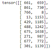
The input of the model is a tensor of shape batch_size x 2, where the first column (x[:, 0]) contains the user IDs and the second column (x[:, 1]) contains the movie IDs.
x,y = dls.one_batch()
x.shape

x[:10,:]
Now we can use a plain Learner class:
model = DotProduct(n_users, n_movies, 50)
learn = Learner(dls, model, loss_func=MSELossFlat())
And fit our model:
learn.fit_one_cycle(5, 5e-3)
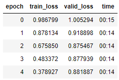
Before getting into the results or looking for improvements, it’s worth looking at the step-by-step architecture in place here.
The dataloaders object contains the input data, and the true scores for each user/movie pair (y).
The model takes the number of users, movies, and factors. Then it transforms them into matrices of user factors and movie factors. Then it dot-products each combination of those. These are the predicted scores.
The learner compares the true scores to the predicted ones, and calculates the loss. It increments the parameters (aka the factors) based on Gradient Descent. Then it recalculates the loss.
The first improvement: force the outputs to range from 0-5 using the sigmoid function. Empirical evidence will denomstrate that setting the range from 0 to 5.5 is more effective.
class DotProduct(Module):
    def __init__(self, n_users, n_movies, n_factors, y_range=(0,5.5)):
        self.user_factors = Embedding(n_users, n_factors)
        self.movie_factors = Embedding(n_movies, n_factors)
        self.y_range = y_range

    def forward(self, x):
        users = self.user_factors(x[:,0])
        movies = self.movie_factors(x[:,1])
        return sigmoid_range((users * movies).sum(dim=1), *self.y_range)

model = DotProduct(n_users, n_movies, 50)
learn = Learner(dls, model, loss_func=MSELossFlat())
learn.fit_one_cycle(5, 5e-3)
At this point we treat each user as equal – but in reality some users are more positive (or negative) than others. We also treat each movie as equal – but in reality some movies are better (or worse) than others.
We have weights, but we need biases. Biases will be a single number for each user and movie that represents the inherent positiveness or goodness of the respective user and movie.
Adjusting our model architecture:
class DotProductBias(Module):
    def __init__(self, n_users, n_movies, n_factors, y_range=(0,5.5)):
        self.user_factors = Embedding(n_users, n_factors)
        self.user_bias = Embedding(n_users, 1)
        self.movie_factors = Embedding(n_movies, n_factors)
        self.movie_bias = Embedding(n_movies, 1)
        self.y_range = y_range

    def forward(self, x):
        users = self.user_factors(x[:,0])
        movies = self.movie_factors(x[:,1])
        res = (users * movies).sum(dim=1, keepdim=True)
        res += self.user_bias(x[:,0]) + self.movie_bias(x[:,1])
        return sigmoid_range(res, *self.y_range)
To run through this architecture in detail again…
We have a matrix of N factors for U users, so that’s a U x N matrix. We have a matrix of N factors for M movies, so that’s a M x N matrix. We have a 1 bias each for U users, so that’s a U x 1 vector. We have a 1 bias each for M movies, so that’s a M x 1 vector.
The function retuns a single score, which is a dot product of the user factors by the movie factors, plus a user bias, plus a movie bias.
The learner then trains on this model:
model = DotProductBias(n_users, n_movies, 50)
learn = Learner(dls, model, loss_func=MSELossFlat())
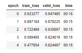
learn.fit_one_cycle(5, 5e-3)
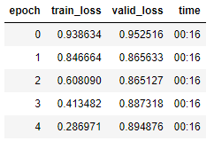
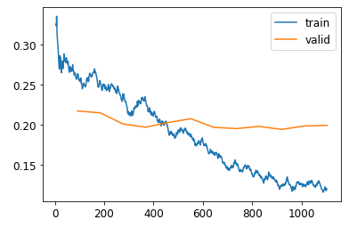
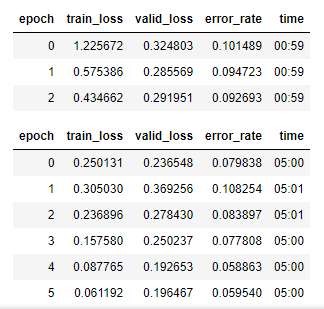
Validation loss gets worse after a few epochs – a sign of overfitting. One way to tackle this is data augmentation, but that’s not possible here. Another is weight decay:
Weight Decay
Weight decay, also called L2 regularlisation, means adding the sum of all the weights squared to your loss function. This will affect the gradients by including a contribution that encourages them to be as small.
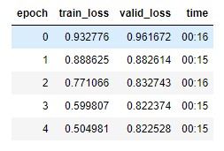
One way to think of overfitting is this: With unrestrained coefficients, the model is free to find extreme values that allow it to jump from observed value to observed value. This makes it fit well on the training data but not so much on the untrained data. This is overfitting in a nutshell. Forcing the model to restrict the values of the coefficients makes for a smoother (and more generalised) fit.
model = DotProductBias(n_users, n_movies, 50)
learn = Learner(dls, model, loss_func=MSELossFlat())
learn.fit_one_cycle(5, 5e-3, wd=0.1)
Creating an Embedding Module
Recreating DotProductBias without using the Embedding class:
Optimisers require that they get all the parameters of a module from the module’s paramter class. If we add a tensor as an attribute to a Module, it will not automatically be included in parameters.
class T(Module):
    def __init__(self): self.a = torch.ones(3)

L(T().parameters())
Wrapping a tensor in the nn.Parameter class tells Module to treat the tensor as a parameter. It will then automatically call requires_grad_.
class T(Module):
    def __init__(self): self.a = nn.Parameter(torch.ones(3))

L(T().parameters())
We can create a tensor as a parameter, with random initialization, like so:
def create_params(size):
    return nn.Parameter(torch.zeros(*size).normal_(0, 0.01))
DotProductBias without Embedding looks like this:
class DotProductBias(Module):
    def __init__(self, n_users, n_movies, n_factors, y_range=(0,5.5)):
        self.user_factors = create_params([n_users, n_factors])
        self.user_bias = create_params([n_users])
        self.movie_factors = create_params([n_movies, n_factors])
        self.movie_bias = create_params([n_movies])
        self.y_range = y_range

    def forward(self, x):
        users = self.user_factors[x[:,0]]
        movies = self.movie_factors[x[:,1]]
        res = (users*movies).sum(dim=1)
        res += self.user_bias[x[:,0]] + self.movie_bias[x[:,1]]
        return sigmoid_range(res, *self.y_range)
Training again:
model = DotProductBias(n_users, n_movies, 50)
learn = Learner(dls, model, loss_func=MSELossFlat())
learn.fit_one_cycle(5, 5e-3, wd=0.1)
How to Interpret Embeddings and Biases
Here are the movies with the lowest values in the bias vector:
movie_bias = learn.model.movie_bias.squeeze()
idxs = movie_bias.argsort()[:5]
[dls.classes['title'][i] for i in idxs]
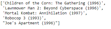
Here’s how to interpret this: These movies are generally not liked, even by people that like similar kinds of movies. We could have sorted movies by their average rating, but that would just tell us if the movie was generally liked. This is telling us that people don’t like watching these movies even if they otherwise enjoy these kinds of movies.
Same now for movies with the highest biases:
idxs = movie_bias.argsort(descending=True)[:5]
[dls.classes['title'][i] for i in idxs]
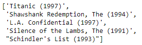
So these are the movies you might enjoy, even if you don’t normally like these kinds of movies.
The embedding matrices have a lot of factors, and it makes it hard to interpret them. Principal Component Analysis can identify the set of vectors that transforms the matrix of embedding factors to a smaller set of factors, while capturing much of the variance of the original matrix. This helps by aggregating correlated embeddings (and therefore similar embeddings).
#caption Representation of movies based on two strongest PCA components
#alt Representation of movies based on two strongest PCA components
g = ratings.groupby('title')['rating'].count()
top_movies = g.sort_values(ascending=False).index.values[:1000]
top_idxs = tensor([learn.dls.classes['title'].o2i[m] for m in top_movies])
movie_w = learn.model.movie_factors[top_idxs].cpu().detach()
movie_pca = movie_w.pca(3)
fac0,fac1,fac2 = movie_pca.t()
idxs = list(range(50))
X = fac0[idxs]
Y = fac2[idxs]
plt.figure(figsize=(12,12))
plt.scatter(X, Y)
for i, x, y in zip(top_movies[idxs], X, Y):
    plt.text(x,y,i, color=np.random.rand(3)*0.7, fontsize=11)
plt.show()
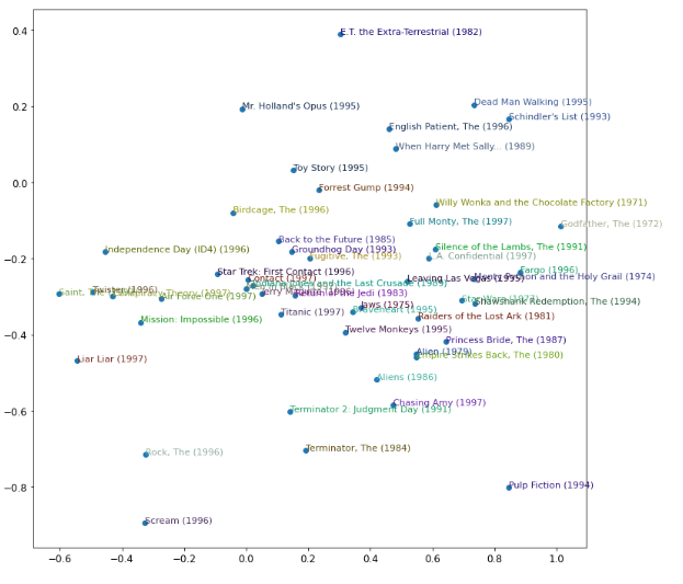
The model is roughly classifying some concept of classic and pop culture.
Using fastai.collab
Fastai’s collab_learner allows us to create and train a collaborative filtering model.
learn = collab_learner(dls, n_factors=50, y_range=(0, 5.5))
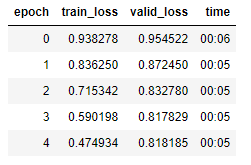
learn.fit_one_cycle(5, 5e-3, wd=0.1)
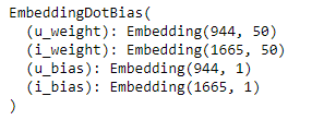
You can print the model to see the names of the layers.
learn.model
Recreating previous analysis
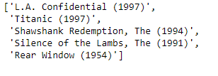
movie_bias = learn.model.i_bias.weight.squeeze()
idxs = movie_bias.argsort(descending=True)[:5]
[dls.classes['title'][i] for i in idxs]
Embedding Distance
We can calculate the distance between embeddings to measure similarity (or lack of it) between movies. The metric is pythagorean distance. In this sense movies are similar if the users that like the movies are similar. The most similar movie to Silence of the Lambs is:
movie_factors = learn.model.i_weight.weight
# idx = dls.classes['title'].o2i['Silence of the Lambs, The (1991)']
# idx = dls.classes['title'].o2i['Forrest Gump (1994)']
idx = dls.classes['title'].o2i['Terminator, The (1984)']
distances = nn.CosineSimilarity(dim=1)(movie_factors, movie_factors[idx][None])
idx = distances.argsort(descending=True)[1]
dls.classes['title'][idx]
Bootstrapping a Collaborative Filtering Model
Great, so you have a trained model. Given a user with a reasonable watch history, you can make recommendations based on similar users’ preferences.
Now, what do you do with a new user? They have no watch history to compare to other users. You could give a new user the mean of all the other users’ embedding vectors. But the mean of the other users’ vectors won’t necessarily make sense. If half the users like horror, and half the users like action, your new user will be recommended half-horror half-action movies.
Another option is to ask a set of questions, then assign an embedding vector based on the answers. This will give some control over the possible enbeddings.
The entire concept of collaborative filtering here is based on users’ ratings. If there are users that rate a lot, they can tilt the system towards their preferences. They can create feedback loops, where their tastes are overrepresented. It’s hard to quantify this overrepresentation though.
Deep Learning for Collaborative Filtering
For deep learning, we can concatenate the results of the embedding lookup. The resulting matrix can be passed through linear layers and nonlinear layers as normal.
Instead of getting the dot product we will concatenate the embeddings. Because of this the matrices can have different sizes. Fastais get_emb_sz returns recommended sizes – aka numbers of latent factors.
embs = get_emb_sz(dls)
embs

Let’s implement this class
class CollabNN(Module):
    def __init__(self, user_sz, item_sz, y_range=(0,5.5), n_act=100):
        self.user_factors = Embedding(*user_sz)
        self.item_factors = Embedding(*item_sz)
        self.layers = nn.Sequential(
            nn.Linear(user_sz[1]+item_sz[1], n_act),
            nn.ReLU(),
            nn.Linear(n_act, 1))
        self.y_range = y_range

    def forward(self, x):
        embs = self.user_factors(x[:,0]),self.item_factors(x[:,1])
        x = self.layers(torch.cat(embs, dim=1))
        return sigmoid_range(x, *self.y_range)
And use it to create a model:
model = CollabNN(*embs)
The Embedding layers are created in CollabNN. embs infers the sizes. self.layers is our mini-Neural Net and in forward we apply the embeddings, concatenate results, and pass through the mini neural net. Then sigmoid_range is applied.
learn = Learner(dls, model, loss_func=MSELossFlat())
learn.fit_one_cycle(5, 5e-3, wd=0.01)
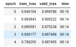
Within fastai.collab, if you use collab_learner and pass use_nn=True it will apply the neural network as part of the collaborative filtering model. The code below makes two hidden layers, of size 100 and 50 respectively:
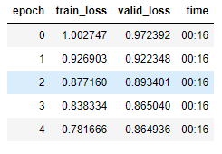
learn = collab_learner(dls, use_nn=True, y_range=(0, 5.5), layers=[100,50])
learn.fit_one_cycle(5, 5e-3, wd=0.1)
Conclusion
This application shows how we can learn the underlying factors within a dataset, and quantify aspects of the data. This can give us information that is otherwise unmeasured.